If you’re building a large spreadsheet in Google Sheets or need to read one that has a hefty amount of data, it’s helpful to apply filters to it. A filter lets you hide specific data (such as numbers or text) inside a range of cells that you select so that you can see what your spreadsheet looks like without this information. In other words, it filters out the data that you don’t want to see in your spreadsheet.
For example, you can design a filter that shows only cells that have numbers that are 50 or greater inside them, and another filter that shows only cells containing numbers of 30 or less. You could then switch between these two filters to see your spreadsheet in these different ways — and then return to your spreadsheet’s original state with its full cell data.
Filters vs. slicers
In Google Sheets, you can refine your spreadsheet’s data using filters or slicers. A slicer does mostly the same thing as a filter, but it’s a toolbar that you embed into your spreadsheet. It makes your spreadsheet a bit more interactive, functioning as a convenient interface that you or others can use to filter cells.
For example, you can set a slicer next to a chart or table to let someone using your spreadsheet quickly remove values from the chart or table and see the filtered results in the chart or table.
Creating a filter
Select a range of data cells in your spreadsheet. In this example, we’ll select C4 to C11.
On the toolbar above your spreadsheet, click Data > Create a filter.
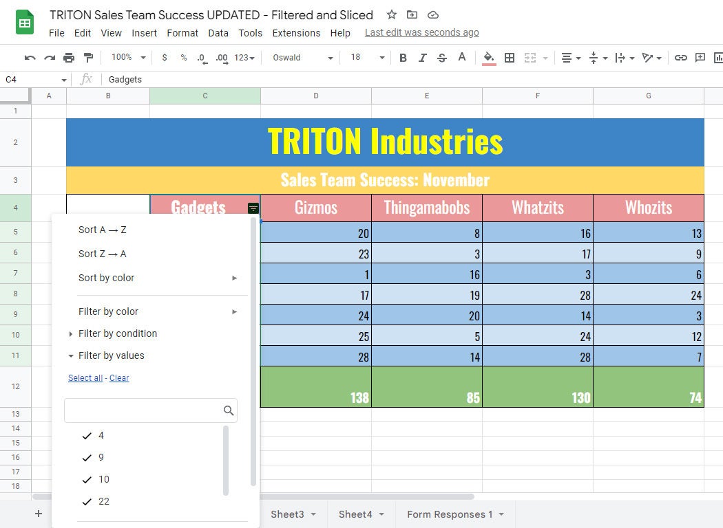
Inside the left, topmost cell that you selected, click the filter (striped triangle) icon. This will open a dropdown panel with sort and filter options.
 IDG
IDGChoose a type of filter to apply to the selected cells. (Click image to enlarge it.)
Sort the order of the selected cell data
The first options you see in this panel are for sorting the selected cells. Unlike using a filter, sorting your data doesn’t actually hide any of the data; it simply rearranges the cells you’ve selected in the order you choose.
You can sort the numbers or text inside the cells (below the topmost selected cell) in ascending or descending order. You can also sort by color if the cell background or text is a different color from your spreadsheet’s default colors.
If you sort the numbers or text via this panel, the action is applied immediately to the cells that you selected for this filter.
Filter the selected cell data
Below the sort options in the panel are the filtering options for the cells you selected. You can filter by color (of the cell background or text), condition, or values.
Filter by values: This option is expanded by default in the dropdown panel. Below the search box is a list of all the values (numbers or text items) in the selected cells, with a checkmark next to each one. (Depending on how many cells you selected, you might have to scroll to see all the values.) Using the search box, you can search for a specific number or text in the range of cells that you selected. You can also use the “Select all” and “Clear” links to check and uncheck all the values at once.
 IDG
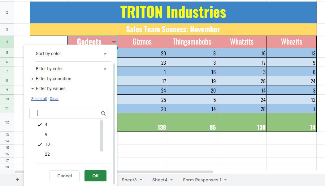
IDGUncheck the values you want to hide from your spreadsheet. (Click image to enlarge it.)
If you uncheck a number or text item in the list below the search box and click OK at the bottom of the panel, the row that contains the cell with the number or text you unchecked will be removed from your spreadsheet. Don’t worry — this row hasn’t been deleted. The filter you created has merely hidden this row, showing your spreadsheet without it.
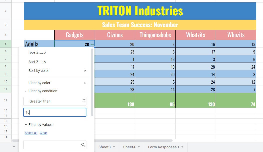
Filter by condition: There are many ways to filter by condition, such as showing only items that contain certain text, items with a certain date, or items with numbers between two particular values. Here’s an example that gives you a basic idea how it works: Let’s filter the selected cells to show only items that contain numbers greater than 10.
Click Filter by condition. Click the box with None inside it. From the long menu list of filter variables that opens, scroll down and select Greater than.
Inside the entry box below “Greater than,” type 10. Scroll to the bottom of the panel and click OK.
 IDG
IDGSpecify the parameters of your conditional filter. (Click image to enlarge it.)
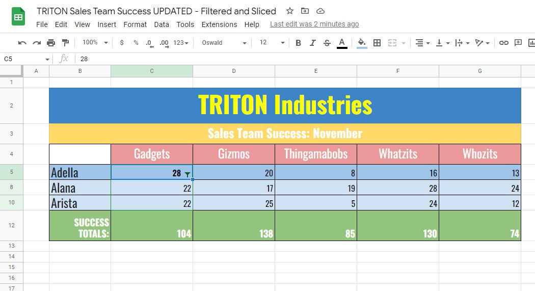
Your spreadsheet now shows only the rows with cells that contain numbers greater than 10. The rows for the cells that contained numbers lower than 10 have been hidden by the filter.
 IDG
IDGThe spreadsheet after the conditional filter has been applied. (Click image to enlarge it.)
Filter by color: If your spreadsheet is formatted with different text or background colors (not simple alternating colors), you can use this filter to show only rows of a specific color.
Click Filter by color, then choose either Fill Color or Text Color from the menu that appears. Select the color that you want to retain. The rows formatted with other colors will be hidden.
Edit a filter
When you apply any filter to your spreadsheet, the striped triangle icon in the topmost selected cell turns into a funnel icon. To adjust what it is filtering, click the funnel icon. This reopens the filter dropdown panel.
Restore your spreadsheet to its original (unfiltered) state
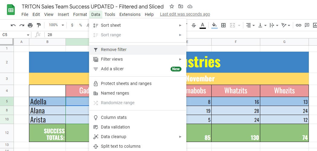
On the toolbar above your spreadsheet, click Data > Remove filter.
 IDG
IDGSelect Remove filter to return the spreadsheet to its original form. (Click image to enlarge it.)
Note: If you used this dropdown panel to sort the cells that you selected for this filter, the actions above will not restore them to their original unsorted state.
Managing your filters
You can give your filter a name and add more filters, each of which can show your spreadsheet in different ways. You can edit the settings for these filters or delete them.
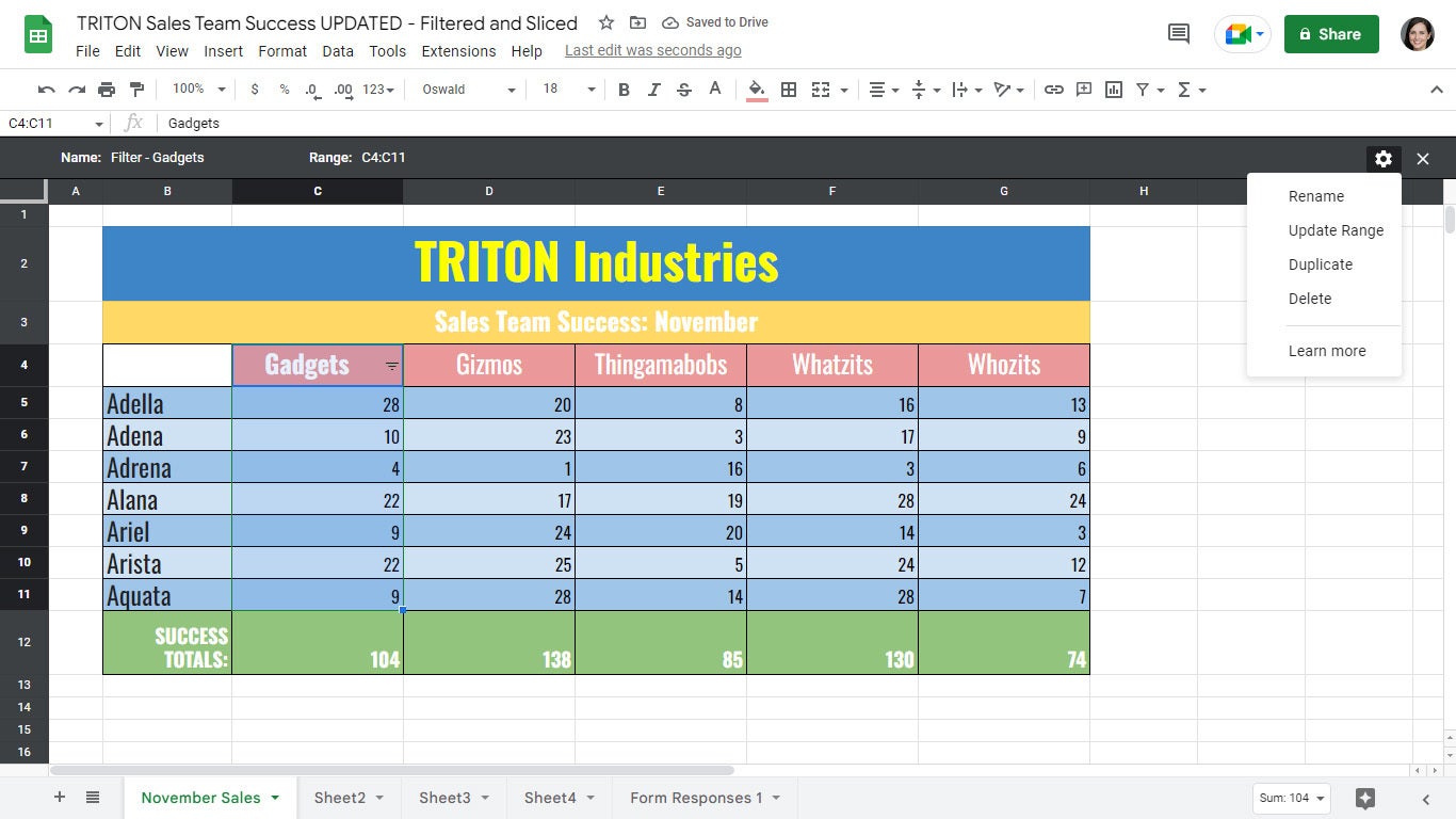
Name a filter: On the toolbar above your spreadsheet, click Data > Filter views > Save as filter view. A black toolbar will appear along the top of your spreadsheet, and your spreadsheet’s columns and row headings will be highlighted in black. This indicates that you’re now in the filter manager.
 IDG
IDGThe filter manager lets you add, edit, name, delete, or take other actions on filters. (Click image to enlarge it.)
At the left of the black toolbar, click inside the entry box to the right of “Name:” and type a name for your filter.
Add another filter to your spreadsheet: Select a range of cells that you want to create a new filter for.
On the toolbar above your spreadsheet, click Data > Filter views > Create new filter view. If you weren’t already in the filter manager, it will appear. Type in a name for your new filter at upper left.
Click the striped triangle icon in the first cell of your new selected cell range and set your new filter’s parameters.
Change the range of cells for a filter: On the black toolbar above your spreadsheet in the filter manager view, click inside the entry box to the right of “Range:” and edit or type a new range of cells for the filter to control.
Exit the filter manager: On the upper right, click the X.
Switch to another filter: By creating and naming several filters in the manner described above, you can switch among them to view your spreadsheet in various ways.
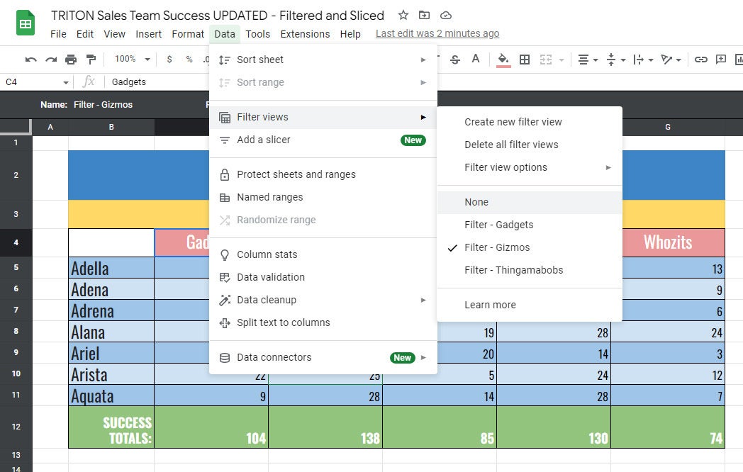
On the main toolbar above your spreadsheet, click Data > Filter views. From the menu that opens, select the filter name. The spreadsheet will appear with that filter applied, and the filter manager will open at the same time.
 IDG
IDGSelect a filter view from the menu to view your spreadsheet with that filter applied. (Click image to enlarge it.)
Duplicate a filter: If you want to create a new filter that’s based on an existing one, open the filter you want to copy in the filter manager (click Data > Filter views and select the filter). Click the gear icon on the upper right, and select Duplicate from the menu that opens. You can then rename and edit the new filter.
Delete a filter: Open the filter you want to delete in the filter manager, click the gear icon on the upper right, and from the menu that opens, select Delete.
Creating a slicer
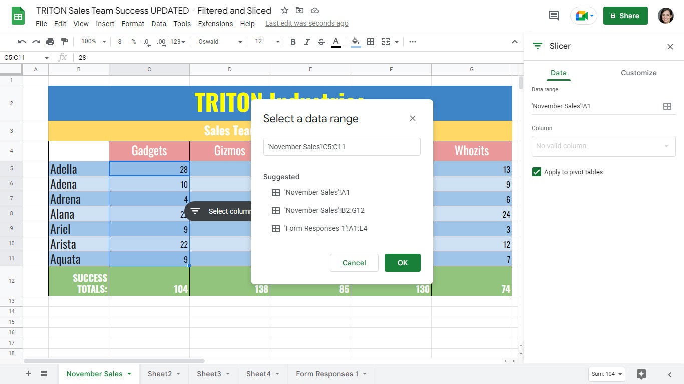
On the toolbar above your spreadsheet, click Data > Add a slicer. The “Slicer” sidebar will open along the right. A panel (“Select a data range”) will appear over your spreadsheet. (If you don’t see this panel, click the Select data range icon (it looks like a grid) on the Data tab in the Slicer sidebar, and the panel will pop up.)
The panel shows suggested data ranges that you can select, or you can click in the spreadsheet and select a range of cells, or select an entire column by clicking the column header. In this example, we have clicked to select C5 to C11 on the spreadsheet.
 IDG
IDGSelect a data range for a slicer. (Click image to enlarge it.)
When you’ve made a selection, click OK, and a slicer toolbar will appear over the spreadsheet.
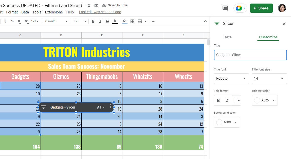
Name the slicer: Let’s give your new slicer a unique name. On the upper right of the “Slicer” sidebar, click Customize and type a new name for the slicer in the “Title” entry box.
 IDG
IDGGive the slicer a unique name. (Click image to enlarge it.)
How to use the slicer toolbar
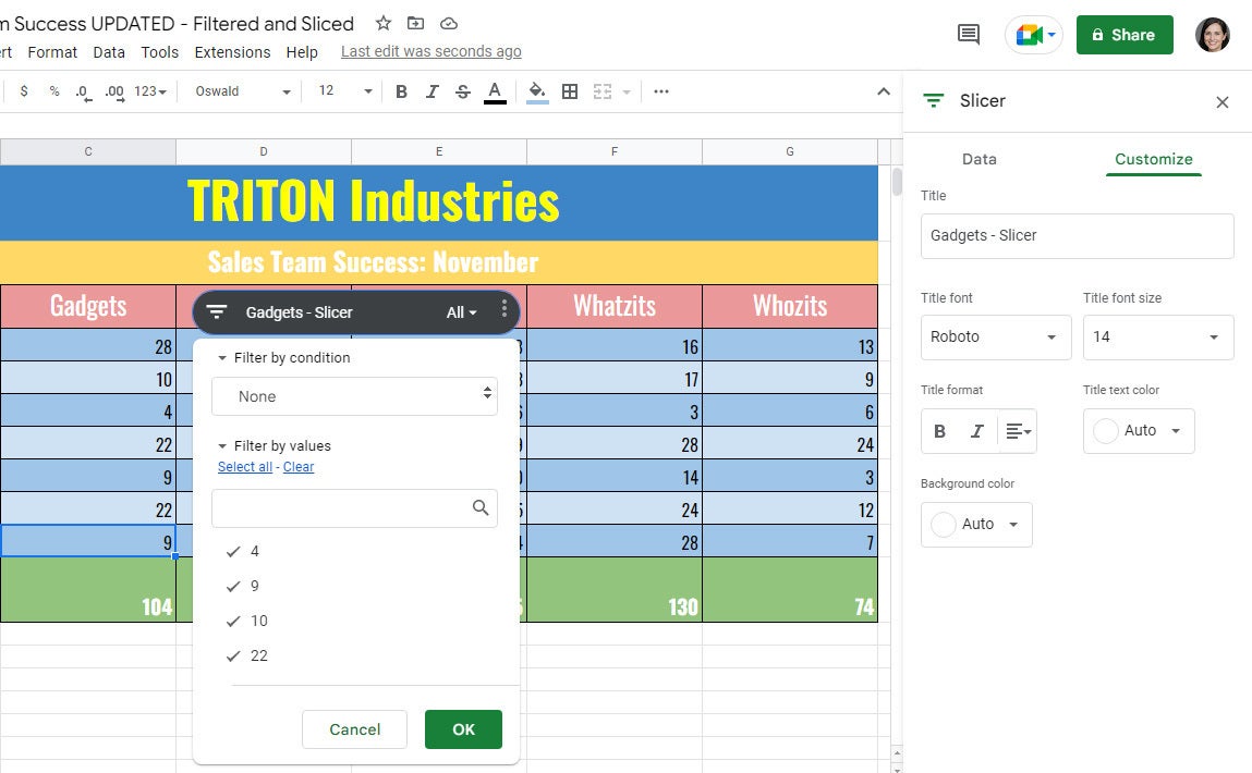
Click the striped triangle icon on the slicer toolbar. This opens a dropdown panel for the slicer that looks and works like the one used to create a filter, but without the options to sort cells or to filter them by color.
The steps outlined above (under “Filter the selected cell data”) for filtering by values and filtering by condition work the same for a slicer dropdown panel.
 IDG
IDGThe slicer toolbar lets you or other users filter the spreadsheet by condition or by values. (Click image to enlarge it.)
To adjust what the slicer is filtering, you or another user can click the funnel icon at the left of the slicer toolbar. Note that the same slicer can filter both by condition and by values.
Managing your slicers
You can edit, copy, delete, move, or resize a slicer. First, click to select the slicer. A frame with eight dots will appear around it.
Resize the slicer: Click and drag one of these dots to resize the slicer to be larger or smaller.
Move the slicer: Click-and-hold the slicer, then drag it to another area on your spreadsheet.
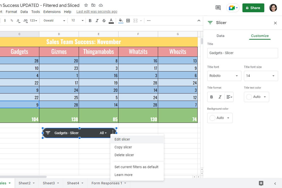
Edit, copy, or delete the slicer: Click the three-dot icon on the upper right of the slicer; from the menu that opens, select the function that you want.
When you delete the slicer, your spreadsheet will be reset back to its original state, showing any cells that were hidden by the slicer.
 IDG
IDGClick the slicer’s three-dot icon to see a menu with further actions. (Click image to enlarge it.)
Set default filters for the slicer: If you want to preserve the filters you’ve set for a slicer so someone else will see the same filtered data by default, click the three-dot icon on the upper right of the slicer and select Set current filters as default from the menu that appears.
Add another slicer: You can add multiple slicers to a sheet, but note that no two slicers can be assigned the same rows of cells. So, for example, your first slicer can be assigned cells that are in rows 1 to 6, but your second slicer can’t be assigned cells in any of these rows.
Copyright © 2022 IDG Communications, Inc.


